Programming Physical Algorithm That Simulates Dam-Break Wave

Introduction 

DamBreak++ wave simulator is a programming environment designed to accelerate the prototyping phase in the validation of numerical algorithms on the so-called Dam Break problem. The software architecture is based on an Object-Oriented framework with a layer of abstract types by which it is possible to extend user applications. A particularly attractive feature is the ability to flexibly combine different numerical algorithms and data structures without disturbing the principal mathematical steps in the calling code. The physicist is often called to test or experiment with different scenarios; this type of environment meets this need. Lately I have been working on migrating from the original version of the library to Modern C++20.

Mathematical and Numerical Model

Physical Algorithm Overview 

This class is at the heart of the programming environment. It is essentially the numerical method under consideration (explicit conservative finite difference scheme). The PhysicalAlgorithm class implementation to numerically integrates the equations governing the simulation. All pieces of the physical algorithm shall be easily exchangeable. Particularly, it is easy to switch between different implementations, for example explicit integrator, or between discretization of spatial terms. 

The framework is intended to provide a programming environment for rapid prototyping. Before running extensive 2D simulation, there is a prototyping phase in which we explore different alternatives. The common practice is validating these numerical schemes on one-dimensional problems that we know the solution to. 

How To Develop a Physical Algorithm 

Framework provides a base class each developer intending to use the Framework will have to provide implementations for. Developed by components, the library provides a rich set of data types that can be used to implement physical algorithms. In this example we use the pointer to function (legacy code). 

‘PhysicalAlgorithm’ base class is abstract and provide a method call ‘calculate’ this is the method user must implement. The numerical model is an explicit conservative scheme (see link above for more details). The right-hand side term are: convective flux, pressure and source terms which include friction and bed slope. Each of these terms must evaluated according to different discretization. For example, flux component may use a Godunov-type flux, pressure terms finite difference derivative.

Solving an ODE system of equastions by an explicit method, you need to evaluate the RHS and to do that there is an abstract class from which you can inherit ‘SweRhsAlgorithm’ to implement the RHS discretization. Once this is done, you must choose an explicit integrator.

Code snippets

Below I present some code snippets of the different components used to implemenet the physical algorithm.

—– ValidateAlgo (inherit from Physical Algorithm base class)

This code snippets show the steps in the computation of the numerical model. This is the physical algorithm.  Numerical model of the equations: the ‘rhs’ algorithm is built and passed to the LDeltaOperator. This operator is responsible for the evaluation (apply discretization).  

void ValidateAlgo::calculate( Sfx::PhysicalSystem* aPhySys)
{
   DamBreakSystem* w_dbSys = nullptr;
   try
   {
     w_dbSys = polymorphic_downcast<DamBreakSystem*>(aPhySys);
   }

...

// RHS disretization (convective flux and source terms (friction and bed slope) 
RhsPtr2FuncFlux w_rhsAlgo{ Sfx::SimulationMgr::getSingleton().getPtrFluxAlgorithmName(),
SimulationMgr::getSingleton().getPtr2FAlgorithm(namPtr2F), w_listDamBreak };

// Physical boundary condition 'H' cond is same as 'A' since Z=0 (flat bed)
PhysicalBoundaryCnd w_phyBCond{};
auto [AbcUpstrm, QbcUpstrm, HbcUpstrm] = w_bndCnd.getBC().first.Values();     // upstream
auto [AbcDwnstrm, QbcDwnstrm, HbcDwnstrm] = w_bndCnd.getBC().second.Values(); //downstream

...
// RHS algorithm boundary cond
w_rhsAlgo.setPhysicalBoundaryCnd(w_phyBCond);

// RHS discretization operator U_t = L_Delta(U;t)  ODE: Ordinary Differential Equations
LDeltaOperator w_Hop{ &w_rhsAlgo}; // set rhs discretization terms

// set operator spatial attributes (derivative order, b.c and so on)
w_Hop.setDerivativType(Sfx::LDeltaOperator::eDxSchemeType::central_2ndorder);
w_Hop.setD1xBCAtBothEnd(Sfx::LDeltaOperator::eDerivBCType::noncentered_2ndorder);

// LDeltaOperator 'apply' method call rhs algorithm to evaluate spatial terms 
Nujic2StepsIntegrator w_Rk2Integrator{ w_U1, w_U2 , &w_Hop };
w_Rk2Integrator.setBCAtBothEnds(w_bndCnd.getBC());
w_Rk2Integrator.setStep(w_CFL*w_timeStep.value()); 
w_Rk2Integrator.step();          // time stepping
// physical systeme state
w_dbSys->setPhysicalState(w_Rk2Integrator.currentState()->asStdVector()); 
w_dbSys->update(); // nodal values update
w_dbSys->setH();   // sections flow update 

// notify our list of section flow
w_dbSys->notify();
}

—– RhsPtr2FuncFlux (inherit from SweRhsAlgorithm base class)

Wrapper legacy code (see my blog …) for more details. SweRhsAlgotihm concept wraps the call to solve or evaluate the spatial terms on the right-hand-side. Numerical model is an explicit conservative form which contains a flux function, source terms which contains derivative.

  SweRhsData<> RhsPtr2FuncFlux::calculate( const Sfx::StateVectorField& aU, const ListSectionsFlow& aListSect) 
  {
   // Numerical flux (convective part)
    dbpp::ff12pair w_FF12 = m_ptr2FuncFF.calculFF( aU.getAfield(), aU.getQfield(),
      PhysicalBoundaryCnd{ m_leftBcNode,m_rightBcNode });

    // pressure term discretization
    [[maybe_unused]] std::valarray<float64> w_PF2(aU.Avalues().size()+1); // first-order derivative
    if( m_usePressure)
    {
      std::valarray<float64> w_U1(aU.Avalues().size() + 1);  // allocate space for ghost node
      std::ranges::copy(aU.getAfield(), std::ranges::begin(w_U1));
      w_U1[0] = std::get<0>(m_leftBcNode.Values()); // 'A' state variable
      w_U1[aU.Avalues().size()] = std::get<0>(m_rightBcNode.Values()); // ghost node
      std::valarray<float64> w_P2(w_U1.size());  // hydrostatic pressure
      // legacy code call pressure numerical algorithm
      BaseNumericalTreatmemt::TraitementTermeP(w_PF2, w_P2, w_U1, static_cast<int>(w_U1.size()));
    }//if-pressure

    // Source treatment (legacy code wrapper) energy slope and bottom slope 
    SbSfTermsEvaluation w_SfSb;
    // return SourceTerms = Sf-Sb ()
    auto w_sfsbArray = w_SfSb.TraitementTermeSource2(aU, aListSect,
      PhysicalBoundaryCnd{ m_leftBcNode, m_rightBcNode });

    using enum FluxTensorMap::eFFcomp;
    // RVO (Return Value Optimization)
    return SweRhsData<> { std::move(w_FF12.first), std::move(w_FF12.second), std::move(w_sfsbArray) };
   }

—– LDeltaOperator (spatial operator)

System of equations can be expressed as ODE system of equations (Ordinary Differential Equations). This operator is responsible for evaluating the spatial terms, i.e. RHS. 

  void* LDeltaOperator::applyTo( const Sfx::FieldLattice& aU1, const Sfx::FieldLattice& aU2)
  {
#ifdef _DEBUG
    SFX_REQUIRE( aU1.values().size() == aU2.values().size(),
      "Field with different size in applyTo()");
#endif
...

// wrapper around legacy code(ptr - 2 - function) RHS discretization
// class dbpp::RhsPtr2FuncFlux (see ValidateAlgp)
 if( m_rhsDiscr) //for this implementation use legacy code ptr-2-func
 {
  // create scalar field
  auto shrGrid1D = std::make_shared<Sfx::gridLattice1D>(Sfx::SimulationMgr::getSingleton().getDBdataTypeStr());
 
 // passing view support move semantic (cheap to move) to intialize scalar field
 auto w_shrdPtrU1 = // takes contiguous range to init scalar field
 std::make_shared<Sfx::scalarField1D>(shrGrid1D,"U1-Field"s, std::views::all(aU1.values().asStdVector()));
      
 auto w_shrdPtrU2 = // takes contiguous range to init scalar field
 std::make_shared<Sfx::scalarField1D>(shrGrid1D, "U2-Field"s, std::views::all(aU2.values().asStdVector()));
      
 // compute RHS according to some wrapper algorithm class to support legacy code
 if( m_rhsDiscr->useSourceTerms() && m_rhsDiscr->isFrictionLess())
 {
   auto w_rhsData = m_rhsDiscr->calculate(Sfx::StateVectorField{ w_shrdPtrU1,w_shrdPtrU2 });
   theRhs->m_S = std::move(w_rhsData.m_S);    // source evaluation
   theRhs->m_FF1 = std::move(w_rhsData.m_FF1); // xvalue (eXpiring value )
   theRhs->m_FF2 = std::move(w_rhsData.m_FF2); // ditto

   return static_cast<void*>(theRhs);
}
 return nullptr;
}
...
}

Technical Report

Technical report (June 2022)

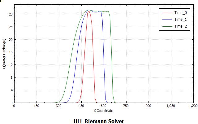
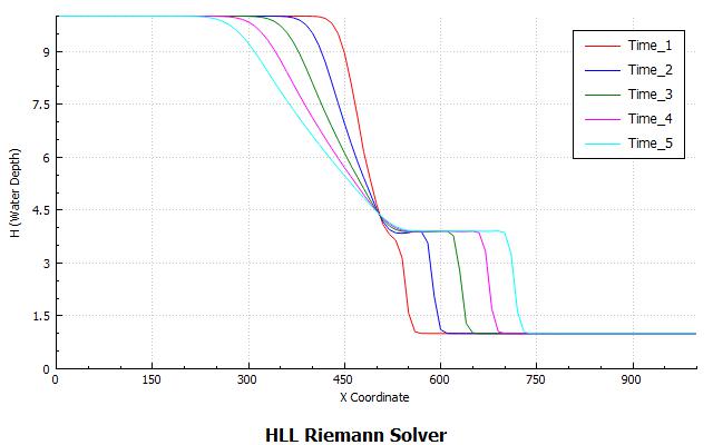
Results

Images below shows the velocity profile and the DamBreak wave propagation at different times.